 How to resolve AdBlock issue?
 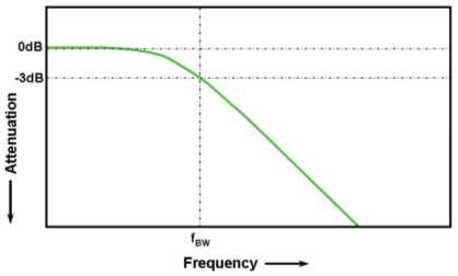 In oscilloscopes or oscilloscope probes, bandwidth is a measure of the width of a range of frequencies measured in Hertz. Specifically, bandwidth is specified as the frequency at which a sinusoidal input signal is attenuated to 70.7 percent of its original amplitude, also known as the -3 dB point. Most oscilloscope companies design the scope/probe response to be as flat as possible throughout its specified frequency range, and most customers simply rely on the specified bandwidth of the oscilloscope or oscilloscope probes, wondering if they are indeed getting the bandwidth performance at the probe tip. Now you can use these step-by-step instructions to simply measure and verify the bandwidth of your probe with an oscilloscope you may already have.
To measure the bandwidth of an oscilloscope probe, a VNA (vector network analyzer) is often used, which is usually expensive and difficult to learn. Also, because typical passive probes are high impedance probes that should be terminated into 1 Mohm of an oscilloscope, it makes the traditional VNA s21 method hard to implement because it is a 50 ohm based system.
The other way to get bandwidth is to use a sine wave source, a splitter and a power meter and sweep the response directly. If you do this, you must set this up to run using a remote interface such as GPIB or USB. Doing it manually is very laborious, subject to mistakes, and requires extensive effort every time you want to evaluate a tweak, etc.
Figure 1 An example of an Oscilloscope Gaussian frequency response
An easier way of measuring probe bandwidth especially for the lower bandwidth probes (<1 GHz passive probe) is the time domain approach utilizing only an oscilloscope with the built-in step signal source, the differentiate function and the FFT. To use this method, your oscilloscope should support the function of another function output. If you can't, an alternative is to pull the time domain waveform data out of the oscilloscope, import it into a PC-based analysis tool such as Matlab, and apply math functions to the step data there.
When you apply a step function to your system, you will get the step response. If you then apply the differentiation (or derivative) to this step response, you obtain the impulse response; then take the FFT of the impulse response to obtain the frequency response of the system.
Agilent’s Infiniium real-time oscilloscope is an excellent tool for this quick bandwidth testing. Here is the step by step procedure of the testing. For this bandwidth measurement example, a N2873A 500MHz passive probe with an Infiniium DSO9404A 4 GHz oscilloscope is used.
Use a performance verification fixture such as Agilent’s E2655C with a 50 ohm BNC cable to connect the Aux output of the oscilloscope to the input of the oscilloscope. The Infiniium oscilloscope has an Aux output port with fast edge speed (~340 psec, 10-90% for Infiniium 9000 Series) for probe calibration. It is very important to note that the rise time of the signal source should be faster than the probe’s rise time and the frequency response of the source is reasonably flat over frequency.
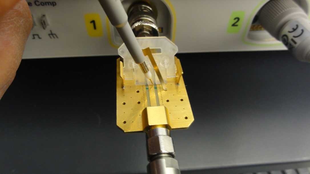
Figure 2 Probing 25 ohm signal source with the Agilent E2655C performance verification fixture
Connect the probe to the PV fixture to measure one edge of the source. Use as short a probe ground as possible to reduce probe loading associated with ground leads.
Ch 1 (yellow) = Source (Aux output) as loaded by the probe
Ch 2 (green) = the measured output of the probe
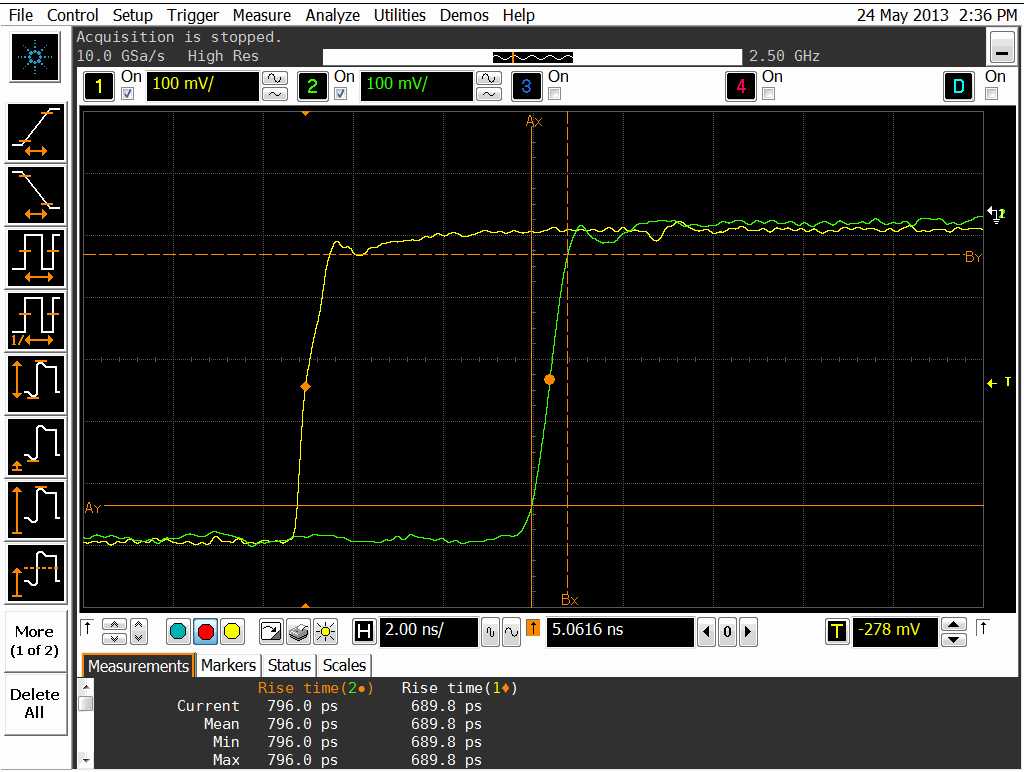
Figure 3 Probing fast edge
Place the rising edges at center of the screen, trigger on the measured output of the probe (ch2) and use averaging, or high resolution acquisition, to reduce the noise on the waveform.
Use the oscilloscope’s built-in math function to differentiate the step response. Now you get the impulse response of channel 2 where the probe is connected. Assign the differentiated output of the step response into the F1 of the oscilloscope.
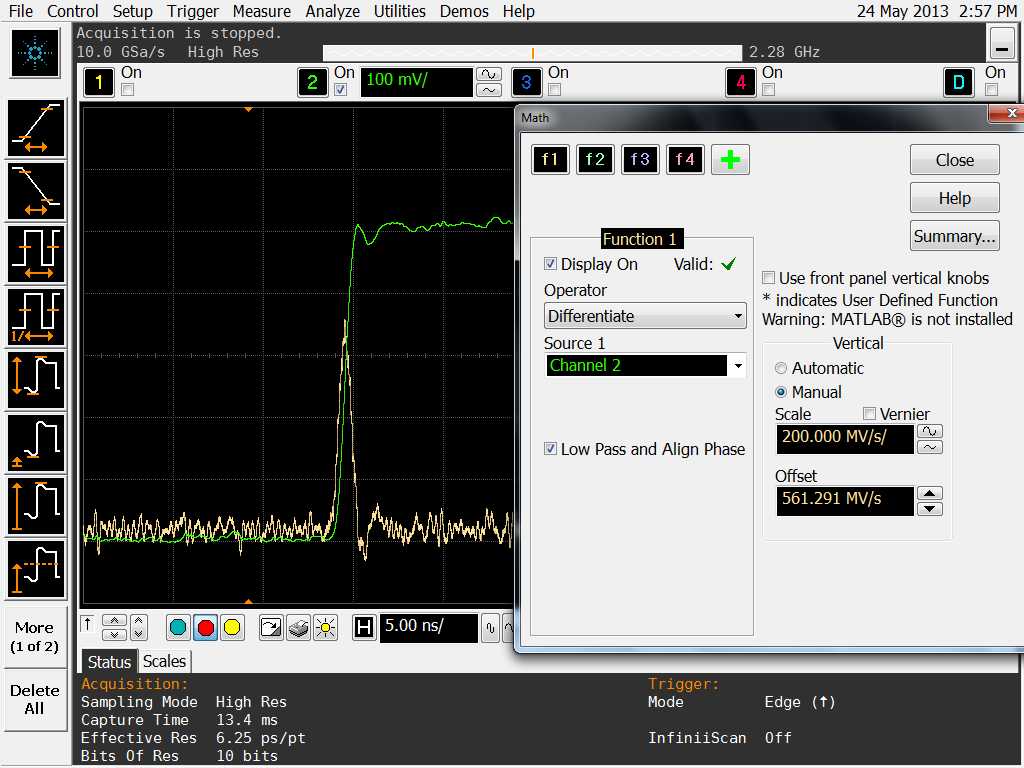
Figure 4 -- Use the oscilloscope’s built-in math function to differentiate the step response.
Apply the built-in FFT Magnitude function on the impulse response (F1) of the measured step signal. Rescale the FFT to 100MHz/div (the center frequency at 500 MHz with the 1 GHz of frequency span across the screen) and 3dB/div vertically.
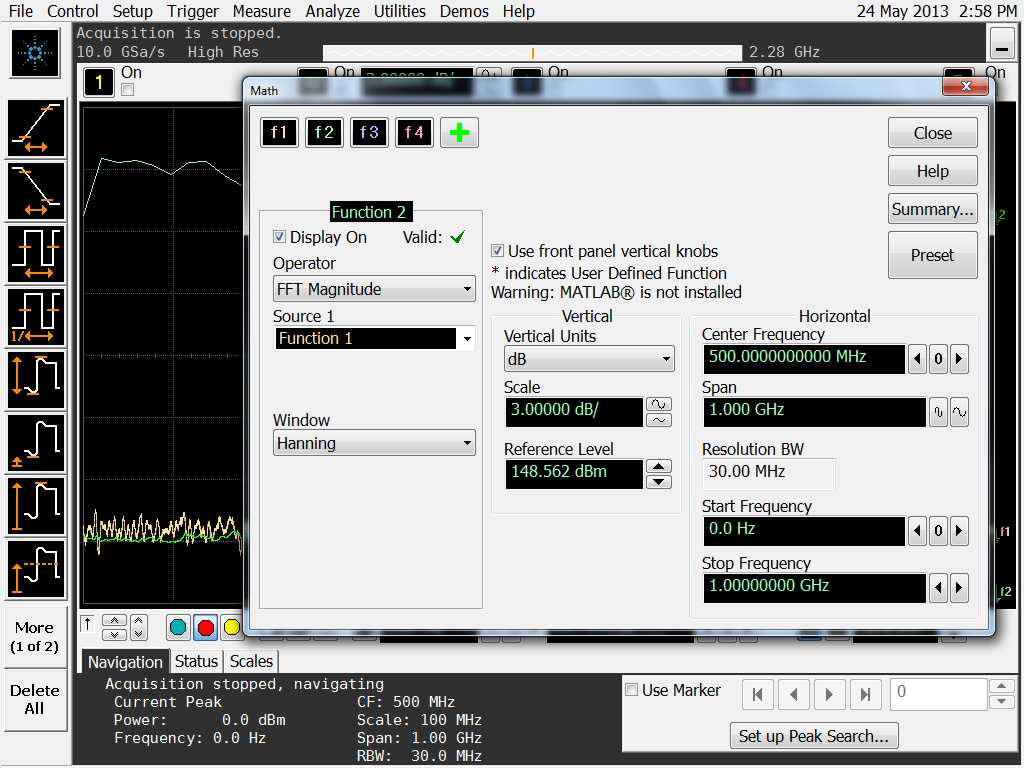
Figure 5 -- Apply the built-in FFT Magnitude function on the impulse response
Now you have a plot of bandwidth. Since the vertical scale of the FFT plot is set to 3 dB/div with the horizontal scale set to 100 MHz/div. You can see the probe has ~530 MHz, as you pick the point in the FFT trace falling by 3 dB.
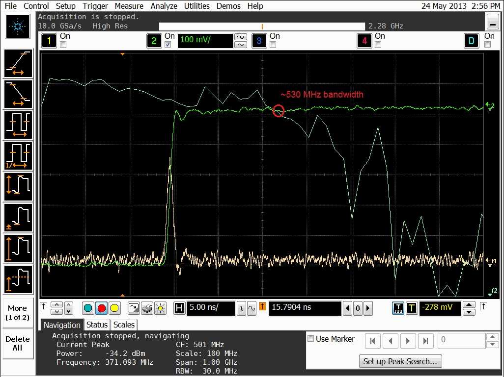
Figure 6 -- Now you have a plot of bandwidth
There is one catch to this. The way we do differentiate in some of the oscilloscopes is taking the best fit slope to three adjacent points and then assigning this slope to the center point. This can really hose the bandwidth measurement up if you don't have enough sample density on the edge, so experiment with sample density and make sure it doesn't affect the bandwidth.
Conclusion
Utilizing the built-in mathematical capabilities available in modern digitizing oscilloscopes, it is possible to derive the frequency response or the bandwidth characteristics of a probe based on the measured step response of a fast step signal. Among those several test methods, the time domain approach is the easiest to duplicate without needing expensive test instruments.
Article based on information from Agilent Technologies.